
Data Science from Concept to Production: A Case Study of Automatic Building Footprint Segmentation
Using Deep Learning and Computer Vision techniques, aerial imagery can be analyzed to automatically predict or augment structure annotations in both form and area...
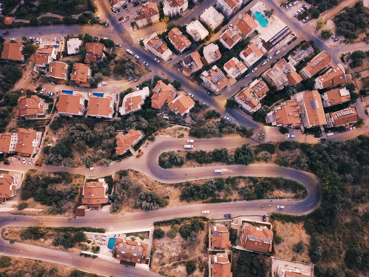
Photo by Ahmet Sali on Unsplash
As satellite imagery has improved over the past ten years, applications of aerial images have dramatically increased. From crop yield to war devastation, these images can tell a detailed story even from a single snapshot. Buildings are perhaps the most common landscape feature in aerial imagery.
Automatic prediction of a building footprint can give rough estimates for both specific and general applications. In general, insights about house size and population density enable broad cross-section comparison of regions. More specifically, determining roof area from a particular building footprint enables a rough estimate of potential work without a tedious outlining process of that building.
Using Deep Learning and Computer Vision techniques, aerial imagery can be analyzed to automatically predict or augment structure annotations in both form and area. As part of my M.S. in Data Science from Regis University, this project employs aerial imagery to automatically predict building footprints from a given latitude and longitude.
SpaceNet Data
Started last year, the SpaceNet challenge open sourced a set of manually labeled building footprints over five regions that includes visible spectrum (3-band), 8-band, and off-nadir tiles. In pursuit of an entire data science pipeline from raw annotated data to production-level API, I have focused on using only the tiles that include the visible spectrum in order to use a global tile-provider for the API.
Due to the 8-week timeline of this entire project, I employed the +250,000 building annotations found in the SpaceNet Rio de Janeiro data set that covers over 2,500 square kilometers. Since they stored the information in a public AWS S3 storage bucket, the 3.4 GB of data was easily downloadable for local exploration of the links, formats, and imagery.
Production-Oriented Approach
Before jumping into the project details, a simple elaboration of my approach will help clarify later discussion. Although my masters focuses on the technical aspects of modeling and data engineering, I am also deeply interested in how to build machine learning (ML) systems end-to-end from data to production since I work for a software firm. Therefore, my entire process has centered around reproducibility, maintainability, and interoperability.
For reproducibility, I have written automated unit tests for most of the core system including data extraction, train/val/test splits, training augmentation, and batch options. This value also extends to the top-level documentation, naming conventions, and accessibility through the command line interface. I have written most of the code to be operable from the abfs command with tasks such as train, evaluate, and export. For the several Jupyter notebooks employed, I have extracted most of the code to external files that can be tested to keep the notebooks as easy to read and up-to-date as possible.
Towards maintainability, I have kept as much as possible to industry code review standards of domain modeling often found in object-oriented systems, in order to facilitate extensions by others and machine learning model changes without rework most of the existing system. For example, when making an polygon API request, it goes through a logical progression of subsystems:
__main__
 -> cli                     # CLI functions
 -> api.server              # Web server entry
 -> api.polygon_prediction  # Top-level handler
 -> api.prediction.lat_lng  # Prediction for coordinates
 -> api.prediction.image    # Prediction from image
 -> keras.Model             # Raw Keras model prediction
For interoperability, I have attempted to keep pieces as independent as possible without compromising functionality. Extensions should be easily achievable as well as integration of the JSON API into any language. Likewise, it should help to define some best practices for next projects. This emphasis on interoperability is motivated by my desire to help standardize the data science process for myself, my co-workers, and the community at large.
Data Preparation
SpaceNet Format
Diving into the Rio data set, all of necessary file references are contained in a single structure called DataConfig. The primary summary file contains the polygons and identifiers to link directly to the processed image tiles. Below is a sample of the first five entries. (See this link for a larger sample.)
| ImageId | BuildingId | PolygonWKT_Pix | PolygonWKT_Geo | geometry | |
|---|---|---|---|---|---|
| 0 | AOI_1_ RIO_img5792 |
1 | ...((408.210... | ...((-43.541... | ...Z ((-43.541... |
| 1 | AOI_1_ RIO_img5792 |
2 | ...((389.833... | ...((-43.541... | ...Z ((-43.541... |
| 2 | AOI_1_ RIO_img5792 |
3 | ...((242.119... | ...((-43.542... | ...Z ((-43.542... |
| 3 | AOI_1_ RIO_img5792 |
4 | ...((311.733... | ...((-43.542... | ...Z ((-43.542... |
| 4 | AOI_1_ RIO_img5792 |
5 | ...((350.582... | ...((-43.542... | ...Z ((-43.542... |
Although some utilities are available from SpaceNetChallenge/utilities, I wanted to understand the data format fully and specifically use only the 3-band (visible spectrum) imagery. After an examination of the geocoded information in those three columns, I found that the PolygonWKT_Pix column is needed to assemble training examples from the tiles. Despite working with GeoJSON previously, I discovered from the utility code that this data is in a Well-Known Text (WKT) format.
As seen in the data folder structure below, the ImageId column corresponds with the TIF images in the 3-band folder. Because the summary CSV contains the WKT polygons, the individual GeoJSON feature files in the vectordata/geojson folder are not required to assemble training examples.
AOI_1_Rio
└── processedData
    └── processedBuildingLabels
        ├── 3band [6940 entries]
            ├── 3band_AOI_1_Rio_img1000.tif
            ├── 3band_AOI_1_Rio_img1001.tif
            └── ...
        ├── 8band [6940 entries]
        └── vectordata
            ├── geojson [6940 entries]
            └── summarydata
                ├── AOI_1_RIO_polygons_solution_3band.csv
                └── AOI_1_RIO_polygons_solution_8band.csv
Additionally, the TIF images include geospatial data that link them directly to a WGS 84 Mercator projection (typically used in GPS). This metadata is extremely important as it will allow converting to and from geographic coordinates when performing pixel analysis.
❯ gdalinfo 3band_AOI_1_RIO_img1000.tif
...
Size is 438, 406
Coordinate System is:
GEOGCS["WGS 84",
    DATUM["WGS_1984",
        SPHEROID["WGS 84",6378137,298.257223563,
            AUTHORITY["EPSG","7030"]],
        AUTHORITY["EPSG","6326"]],
    PRIMEM["Greenwich",0],
    UNIT["degree",0.0174532925199433],
    AUTHORITY["EPSG","4326"]]
...
Corner Coordinates:
Upper Left  ( -43.7125239, -22.9499059) ...
Preprocessing
Because the goal here is more than just drawing a bounding box around buildings, an image segmentation approach is critical for determining an exact polygon. For a given pixel, therefore, the model should predict whether it is part of a building. For preprocessing, pixel-based predictions mean that the polygons need to be "stamped" into a single image to create a mask of black and white pixels where the white pixels indicate the buildings.
Creating these pixel masks from the polygons was perhaps one of the most difficult steps of the preprocessing due in part to the Python to C++ interop with osgeo and the lack of internet resources for how to use the Python library properly. For example, simply refactoring the method into multiple calls often caused a segmentation fault (not to be confused with image segmentation) because C++ had released the memory despite Python still needing it to exist.

Exploratory Data Analysis (EDA)
With the initial data preprocessing in place, I explored the data a bit further in a Jupyter notebook. Having imported the PolygonWKT_Geo data as shapely objects, the area of each building is calculated via a degrees to feet projection. Using a few matplotlib and seaborn commands, a visualization of the area distribution reveals a healthy cross-section of the data.
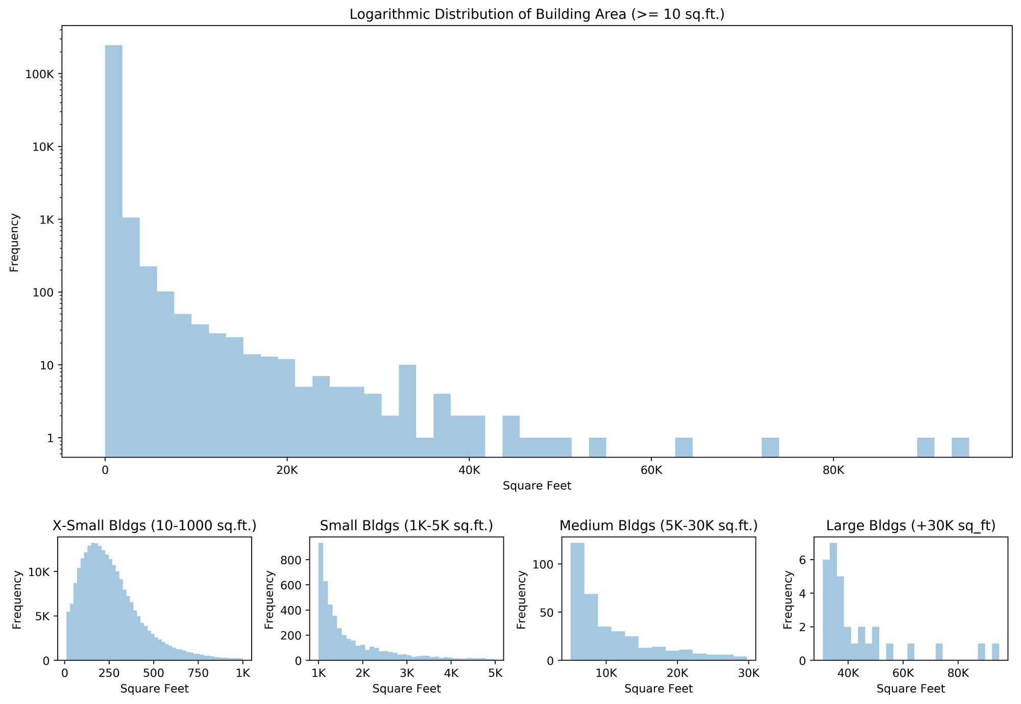
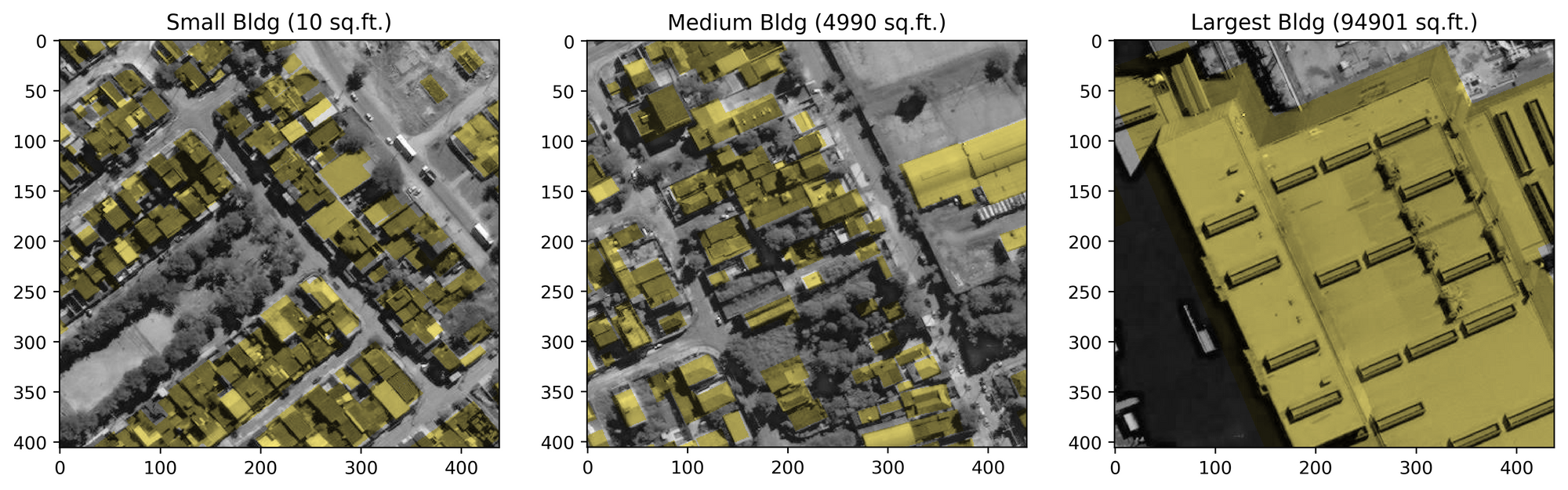
From these graphs, the median of 227 square feet is seen in the smallest building category. As it turns out, 98.1% of the buildings are under a thousand square feet. To determine how these actually appear relative to the tiles, labels overlaid onto the aerial imagery for buildings from several categories give a decent sample of the proportions.
Because the EDA forced a calculation of building area, I opted to model only on the tiles with buildings (>= 0 square feet) since the intended use of the API is for a requested building location.
Modeling
Before actually writing the neural network, I still had several tasks to complete. Keras expects to be handed batches of inputs and outputs (as numpy arrays) unique to the given test split (train/validation/test). To this end, I updated the Data class and and created a generic GroupDataSplit class to manage data splits and create data frames for each phase (train/val/test). Because the Keras generator worked extremely well for previous projects, I created an extension to this system with a class called Generator that inherits from keras.Sequence and simply provides the interface expected. I also implemented segmentation augmentation that optionally creates "new examples" by rotating and scaling the tiles and the associated labels.
With all of this behavior unit-tested and ready for prime time, the model setup becomes extremely easy to discern.
# Use Rio 3band data
config = DataConfig(DEFAULT_DATA_DIR, BAND3, RIO_REGION)

# Train (70%), Val (10%), Test (20%), Fixed seed
split_config = DataSplitConfig(0.1, 0.2, 1337)

# Create data with batch size
data = Data(config, split_config,
            batch_size=args.batch_size,
            augment=True)

# Exclude empty polygons
data.data_filter = lambda df: df.sq_ft > 0

# Create model
# ...
These are just some of the features that have now been enabled:
- Consistent split of data (doesn't change between runs)
- Train data randomization
- Train data augmentation
- Filtering data examples
- Scaled inputs
- Configurable batch size
- Configurable input data image size
- Keras integration
U-Net & Training Process
For the modeling process, I was eager to experiment with fully-convolutional neural networks, particularly the U-Net architecture. After a bit of tweaking and discussion with my professor, I added layers through the training process until I reached my 5-level deep U-Net with 31,032,837 parameters and frequent 25% dropout layers. I experimented with different hidden activation functions, kernel initializers, and fewer layers. With this architecture, the highest level features are max-pooled into a 32x32 filter before being up-sampled to the original size after being combined with the relevant skip connections.
For network input and output, I began with a 512x512x3 input and predicted a 512x512 mask of building probabilities by pixel using a sigmoid activation with an SGD (stochastic gradient descent) optimizer. As will be later seen, these decimal values will need to be converted to polygons for actual use from an external application. For the convolutional layers, I used an he_normal kernel initializer for the initial weights, which samples from a truncated gaussian distribution.
To facilitate the training process, I employed a TensorBoard callback that plots the network loss, metrics, and even a custom image visualization of validation set examples. This visualization was a key element from one of my computer vision projects last year that revealed a Keras issue only late in the semester because I didn't put a visualization together earlier. Although it wasn't 100% effective, it did give a bit of sanity check to the network training before the official evaluation step.
As seen above, the green corresponds to where the pixels were correctly predicted, the red to where it mistakenly predicted a building, and blue to where it missed an actual building. Combining this visualization with TensorBoard's scalar graphs, I had good insight into the training progress (even remotely).
For metrics, I attempted several variations of binary mean intersection-over-union statistic. After writing my own as well as trying to the TensorFlow implementation, I eventually abandoned it in favor of the SpaceNet metric of an F1-score for my final evaluation. However, by monitoring the binary cross-entropy loss function in tandem with the image validation in TensorBoard, I was still able to accurately experiment with the network hyperparameters.
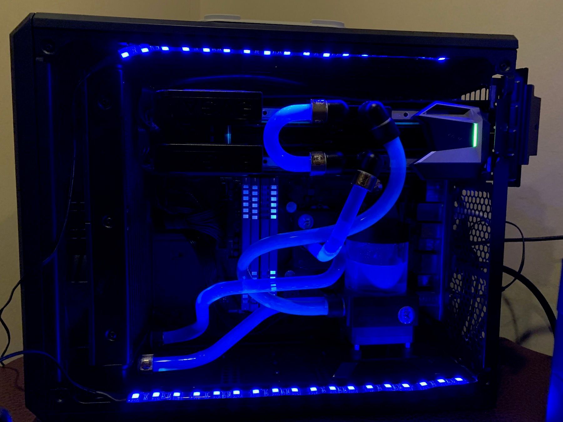
Through the training process, I experimented with different epoch sizes. Although the training data was both shuffled and augmented during each epoch, training on the entire 755 batches (8 per batch) for a single epoch more quickly achieved convergence. This experiment was made possible by training across two 1080 Ti's. During the course of the project, I installed liquid cooling to keep the temperatures down on both GPUs (from 91°C to 69°C for training).
Because of my background in software engineering, I knew that my biggest opportunity for learning would be during the modeling process. To this end, I created a CLI for the basic training in order to more quickly experiment with various hyperparameters.
❯ abfs train -h
Using TensorFlow backend.
usage: abfs train [-h] [-lr LEARNING_RATE] [-s SIZE] [-e EPOCHS]
                  [-b BATCH_SIZE] [-mb MAX_BATCHES] [-gpus GPU_COUNT]

optional arguments:
  -h, --help            show this help message and exit
  -lr LEARNING_RATE, --learning-rate LEARNING_RATE
  -s SIZE, --size SIZE  Size of image
  -e EPOCHS, --epochs EPOCHS
  -b BATCH_SIZE, --batch-size BATCH_SIZE
                        Number of examples per batch
  -mb MAX_BATCHES, --max-batches MAX_BATCHES
                        Maximum batches per epoch
  -gpus GPU_COUNT, --gpu-count GPU_COUNT

❯ abfs train -lr 0.02 --batch-size 8 --epochs 150 -gpus 2
...
Results
Evaluation
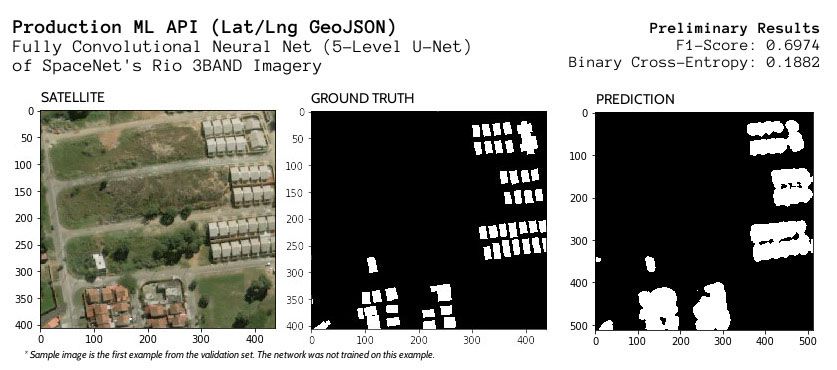
According the example SpaceNet implementation for building extraction from the Rio data set that I found after my modeling, they achieved an F1-score of 0.729 on the entire public data set. My raw F1-score was 0.692. However, there are several key differences that distinguish my work.
- My model was trained using only the 3-band imagery. The example uses both 3-band and 8-band imagery.
- My model employed with a 60-10-20 split (60% train, 10% validation, 20% test). The example was evaluated on the entire public data set (and does not state what it was trained on).
- My model filters out tiles with no buildings. The example does not seem to filter out any examples.
However, mu final F1-score metric is not directly calculated from the network training process. This raw F1-score is a combination of the probabilities. To actually produce polygons, the model must use a threshold to find the relevant contours in the mask image.
Tune Tolerance
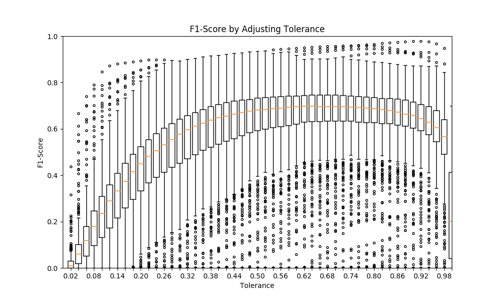
Although the threshold tolerance is not directly implemented in the neural network, it is still a parameter that must be tuned. Using the validation data, the output masks of varying grey-to-white pixels must therefore be converted at different tolerances (1 - threshold) to binary white/black pixels. Once converted, each sample can then be assessed with the F1-score metric. However, it is not simply enough to choose the highest median F1-score. By visualizing these distributions as a series of box plots (see figure below), the best tolerance can be manually determined as well as programmatically found via a combination of high median and low standard deviation.
As seen in the tuning notebook, this calculation can be quite computationally expensive. I started with a CPU implementation that was going to take about an hour and cut it down to to 7.4 seconds by writing it in TensorFlow using CUDA. Below is a sample run on the selected model.
❯ abfs tune -w checkpoints/unet-f63fce-0024-0.19.hdf5 -gpus 2
Calculating F1-Scores... This may take perhaps even an hour if no GPU.
F1-Score calculation complete: 7.39 seconds
Plot has been saved to /tmp/tmp_xjeqphr.png. Please open to view.
Tuned tolerance: 0.70 w/ median=0.6974 stdev=0.1722
From this tuning process, the final F1-score was 0.6974.
Building a GeoJSON API
With the model built, I crafted a pyramid web server with two API endpoints–one that returns the raw masked image with the varying gray pixels and the other one that uses the tuned tolerance parameter to create and return GeoJSON polygons.
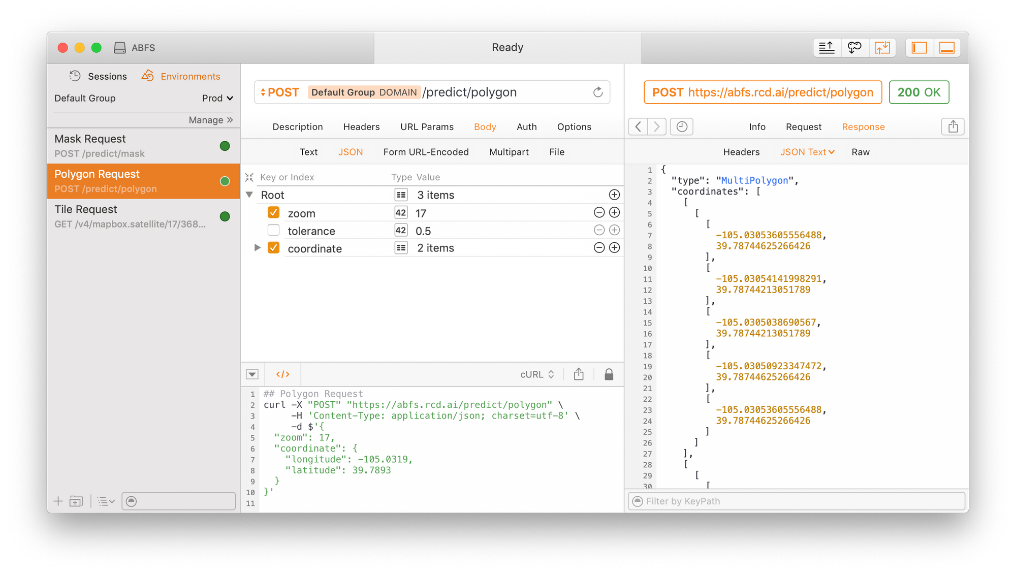
As previously mentioned, my goal was to swap out the tile provider from SpaceNet to one that I could map directly from latitude and longitude. To this end, I employed MapBox since I could easily stay with their free limits for testing this project.
Since the focus of this project is not primarily the software engineering, I will avoid details of the pixel-to-coordinate projection mapping and GeoJSON creation. Like the other parts of this project, the server is easily accessible and configurable from the CLI.
❯ abfs serve -h
Using TensorFlow backend.
usage: abfs serve [-h] [-w WEIGHTS_PATH] [-ws3 WEIGHTS_S3] [-m MODEL_PATH]
                  [-ms3 MODEL_S3] [-a ADDRESS] [-p PORT] [-mb MAPBOX_API_KEY]
                  [-t TOLERANCE]

optional arguments:
  -h, --help            show this help message and exit
  -w WEIGHTS_PATH, --weights-path WEIGHTS_PATH
                        Path to hdf5 model weights
  -ws3 WEIGHTS_S3, --weights-s3 WEIGHTS_S3
                        S3 path to hdf5 model weights
  -m MODEL_PATH, --model-path MODEL_PATH
                        Path to keras model JSON
  -ms3 MODEL_S3, --model-s3 MODEL_S3
                        S3 path to keras model JSON
  -a ADDRESS, --address ADDRESS
                        Address to bind server to
  -p PORT, --port PORT  Port for server to listen on
  -mb MAPBOX_API_KEY, --mapbox-api-key MAPBOX_API_KEY
                        Mapbox API key
  -t TOLERANCE, --tolerance TOLERANCE
                        Default tolerance parameter (output from tune)
Deployment to Production
Using environment variables in tandem with this CLI, I set out to create an entire CI/CD pipeline. For unit testing, I created a public project on Semaphore CI to automatically test for code regressions. After many failed production attempts (or excessively expensive options) with AWS Lambda, Heroku, and a Python environment on AWS Elastic Beanstalk, I succeeded with a Docker container that runs the necessary environment in Elastic Beanstalk.
Although I am sure that most Python projects with work with the stock Python environment, this project required certain versions of C-based libraries to be installed for the geospatial calculations. For the minimum processing requirements, I used a t2.medium EC2 instance that returns the API results in about 11 seconds. For reference, my GPU-build performs it in 900ms and my Mac (no CUDA) returns in 4 seconds on its i9 6-core CPU. For $33 a month, the t2.medium instance was a reasonable option for testing this public API.
Conclusion
The last eight weeks has held a significant amount of learning. From a data science pipeline perspective, I was able to go from raw data to production. Although the model could certainly be tuned further, model improvements should not require a significant amount of change to the system even if an entirely different network is selected.
In consideration of further efforts, one of the elements that the model could not take into account is different environmental settings. When, for example, I ran it in my home state of North Carolina, the heavy vegetation seemed to throw it off. My preliminary theory is that model's data source of Rio looks significantly different from an aerial perspective with its commonly dusty streets, packed houses, and little vegetation. Solving this problem would likely require artificial augmentation (adding trees and masking obscured labels) or tiles from a different region. Additional work in this direction should significantly improve the model's ability to generalize.
Considering the network itself, I only had the time to explore the U-Net architecture. Pursuing a different approach with perhaps an auto-encoder or XGBoost would likely be helpful. Of course, ensembling these models would likely improve the accuracy. Aside from the model improvements, performance optimization would be a significant prerequisite to employing it in a client project or as an external API.
If you've read this far, then congratulations! I appreciate the interest. If this particular project seems beneficial to you or a project of yours, feel free to drop me a note at rcddeveloper@icloud.com or checkout the entirety of the source code at github.com/rcdilorenzo/abfs. 🌟 Please star the repository to show your appreciation! 🎉

Comments ()