
Eye Tracking: Activation Functions
While experimenting with multiple architectures, I took the opportunity to step back and consider how I might confine the output of the neural network to be a bit more specific to the GazeCapture of iOS devices.

Photo by Joshua Sortino on Unsplash
This blog post is weekly update from a project I've been working on as part of my graduate studies at Regis University for an M.S. in Data Science. Visit the repository for more details.
This week has been filled with fluctuating loss values ranging from <100 to >1,000,000,000 which has made my progress a bit discouraging. However, while experimenting with multiple architectures, I took the opportunity to step back and consider how I might confine the output of the neural network to be a bit more specific to the GazeCapture of iOS devices. Because I performed an initial exploratory data analysis (EDA) of the data, I already knew that the maximum extents of XCam and YCam values that measure the distance in centimeters from the lens. (In this case, this maximum distance is the measure from an 12.9" iPad Pro's lens to its furthest corner.) This can be clearly seen by the following extract from the EDA notebook.
| dotInfo.XPts | dotInfo.YPts | dotInfo.XCam | dotInfo.YCam | |
|---|---|---|---|---|
| count | 2258008.00 | 2258008.00 | 2258008.00 | 2258008.00 |
| mean | 294.22 | 260.50 | 0.12 | -1.85 |
| std | 200.75 | 190.86 | 6.08 | 4.87 |
| min | 40.00 | 40.00 | -26.52 | -26.52 |
| 25% | 139.73 | 116.07 | -3.72 | -4.23 |
| 50% | 261.64 | 220.00 | 0.40 | -1.24 |
| 75% | 414.28 | 335.00 | 3.67 | 0.94 |
| max | 1326.00 | 1326.00 | 26.52 | 26.52 |
However, at this point, the neural network was simply using a linear function, thereby producing any value from (-∞, +∞) since it just passed the value of the last neurons as the network output. Although the eye tracking project might be theoretically extended to show really "wherever" the person is looking, it is technically limited by this data set to values between [-26.52, 26.52] for both x and y.
Determining a Custom Activation Function
So, we know that the network should never actually produce values outside of the [-26.52, 26.52] range. The question is: How should the coordinate output layers be constrained? Should it just cap the values at that extent? The reality is there are several requirements for the optimal function being sought:
- Restricts the range. The goal is to predict where a person could be looking as constrained by an iOS device, not anywhere in space. The function should therefore cap at somewhere near
26above and below zero. - Must be differentiable. Although there are activation functions that are not "technically differentiable" can be used such as ReLU, keras can do the differentiation automatically if given a nicely-behaved function.
- Accepts a wide domain to product values less than the extents. For example, if a step-wise function were used, only the maximum or minimum values could be produced. This requirement is that a wide number of values can be used to product values well within the possible range.
To determine what function might work, the sigmoid function is a great place to start. Although it is typically used as an activation function for classification problems, it might be easily adjusted to fulfill our requirements. Below is an example of the base sigmoid function.
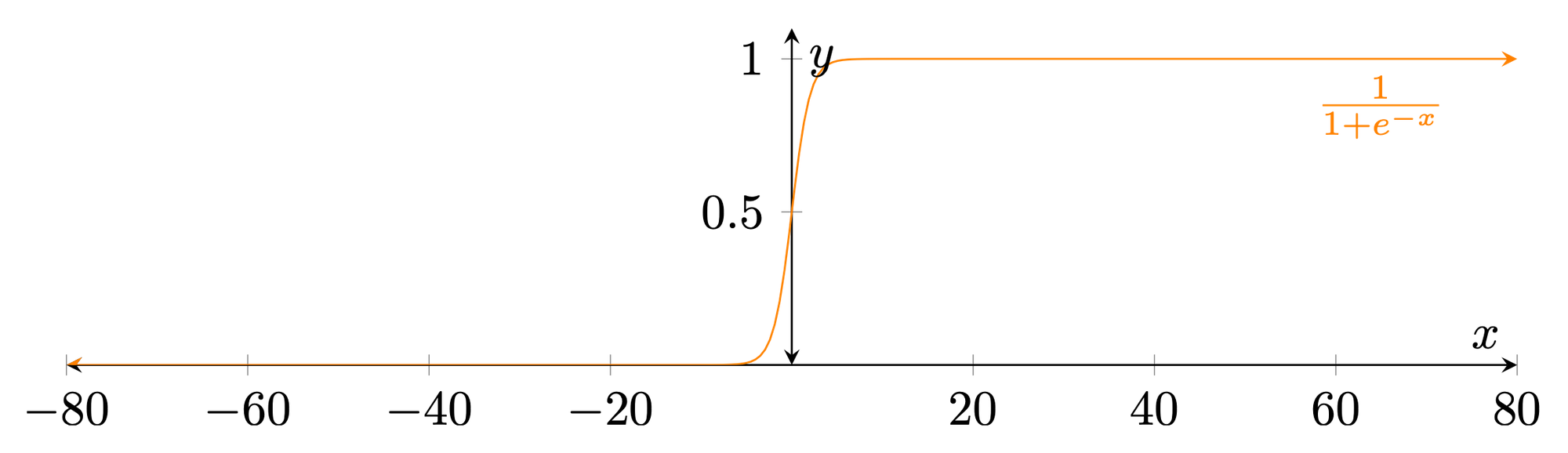
Even without modification, this activation function caps the range, is differentiable, and produces values less than its extents. However, the range still needs to be adjusted and a larger range of x-values should be accepted to produce values less than the maximum extent. Thankfully, the Wikipedia article on sigmoid functions also listed a graph of similar functions submitted by an extremely helpful contributor (as seen below).

Armed with the basic sigmoid function and other "logistic-like" functions, I was able to quickly experiment with some different functions using the built-in Mac utility Grapher. Below are the many variations I graphed for experimentation.
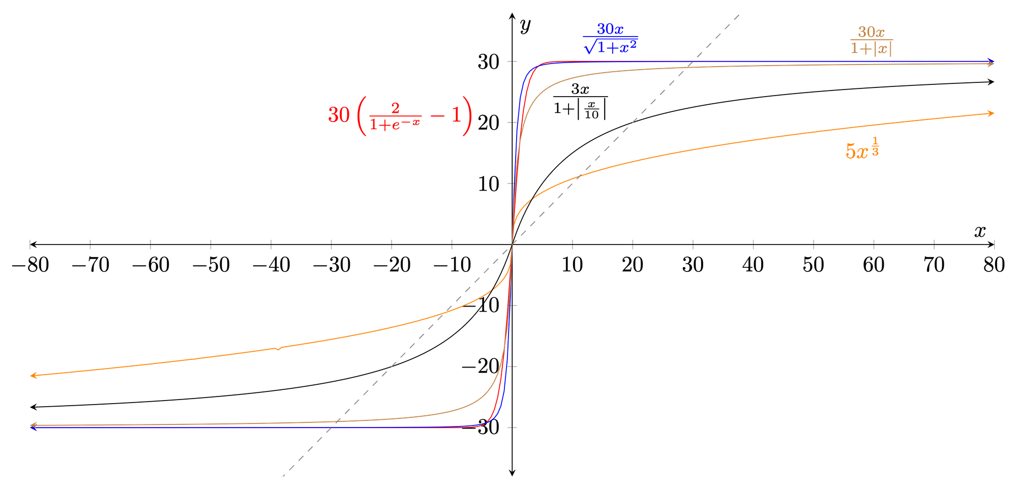
Looking at these functions, several qualities are apparent. The cubic root function (in orange), although producing a good range of outputs, does not actually cap the range. On the other end of the spectrum, the modified sigmoid function (red) and its square root counterpart (blue) properly cap the extents at 30 but only accept values between approximately -5 and +5 to produce anything aside from the maximum extents. However, the base absolute value equation (brown) and its variant (black) overcome this problem since they accept values beyond even -80 and +80 that product values less than the maximum extents.
Conclusion and Results (Ongoing)
Sticking with the absolute value equations as variants to test, I immediately saw the neural network loss values in a friendlier neighborhood (<2000). However, as the activation function is only one of the myriad of hyperparametrs that can be changed for the network, my analysis continues in an effort to have the loss actually converge to a local minima without continuously changing.
Hopefully, this article has given you an idea of how activation functions might be tweaked for your use case. Although the common ones will often suffice (Leaky ReLU, Softmax, Sigmoid, etc.), sometimes a custom activation function is needed because of the given problem's specificity.
Thoughts? Comments? Do you use custom activation functions for certain regression problems? I'd love to hear from you in the comments below.


Comments ()