Background

As a part of my graduate studies at Regis University, I have had the opportunity to begin exploring my own project during my Deep Learning class. (Data Source) By using this data set before my practicum (Spring 2019), I hope to not only explore and model some interesting data but also be prepared to solve the eye tracking problem by combining known solutions as well as current research in Deep Learning (e.g. synthetic data training, JavaScript Convnets, pre-trained model adaptation) and thereby bring some of the concepts presented by Krafka et al. (2016) to the web.

Repository: https://github.com/rcdilorenzo/msds-686-eye-tracking

Begin Then Backtrack

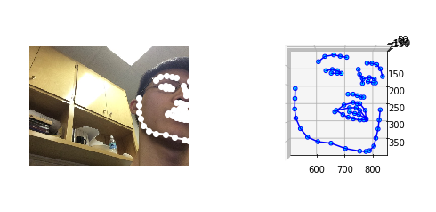
After discovering the face-alignment project several weeks ago, I ran it against the entire 2.4M images available in the GazeCapture data set. Below is a sample of the output of Adrian Bulat's deep neural network (written using PyTorch).

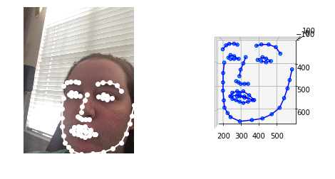
For my purposes, I focused this week on modeling the predicted (x, y) distance from the camera lense based on the output of the facial landmarks (68 points in 3D space) as well as the cutout images of each eye. After much debugging in my attempts to coerce the dimensional shapes of the keras layers to cooperate, I found that I could only combine the left and right eye images with the (x, y, z) points of the face-alignment library by having a predefined input shape for each eye. To this end, I spent some time backtracking to produce a consistent 128x128 pixel image (as seen below).

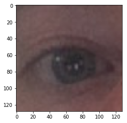
Although I was basing each eye image off of the coordinates from the face-alignment library, I had to do some resizing to make sure that I had a consistent input size. Accomplishing this resize with tensorflow turned to not be the difficult part. The issue primarily arose with images where the projected face landmarks indicated that at least one of the eyes was not even visible in the image. This meant that I needed to still produce a 128x128 image since my neural network would expect that as an input. For the tensorflow code, therefore, I required at least a 1x1 pixel image was sliced off from the image based on the coordinates before being scaled to the appropriate size.

Thankfully, I was able to backtrack a bit to and revamp the input preparation such that the network could reliably depend on only 128x128 images for the right and left eyes. Below is the tensorflow code for extracting a single eye from the image and landmark points.

def eye_tensor(image, predictions, factor, index = LEFT):
    eye_points = predictions[index:(index + 6), :]
    x = eye_points[:, 0]
    y = eye_points[:, 1]

    # Image dimensions
    image_shape = tf.shape(image)
    image_height = image_shape[0]
    image_width = image_shape[1]

    # Find bounding box
    min_x_raw, max_x_raw = tf.reduce_min(x), tf.reduce_max(x)
    min_y_raw, max_y_raw = tf.reduce_min(y), tf.reduce_max(y)

    # Expand by factor and reform as square
    width = tf.to_float(max_x_raw - min_x_raw)
    height = tf.to_float(max_y_raw - min_y_raw)
    sq_size = tf.to_int32(tf.round(tf.reduce_max([width * factor, height * factor])))

    # Compute deltas
    width_delta = tf.to_int32(tf.round((tf.to_float(sq_size) - width) / 2))
    height_delta = tf.to_int32(tf.round((tf.to_float(sq_size) - height) / 2))

    # Pre-compute max_x and max_y
    max_x = max_x_raw + width_delta
    max_y = max_y_raw + height_delta

    # Calculate whether eye visible within image
    both_eyes_visible = tf.logical_and(max_x < image_width, max_y < image_height)

    # Update frame based on delta (but with min/max boundaries)
    max_x = tf.reduce_min([tf.reduce_max([max_x, 1]), tf.shape(image)[1]])
    min_x = tf.reduce_max([tf.reduce_min([min_x_raw - width_delta, max_x - 1]), 0])
    max_y = tf.reduce_min([tf.reduce_max([max_y, 1]), tf.shape(image)[0]])
    min_y = tf.reduce_max([tf.reduce_min([min_y_raw - height_delta, max_y - 1]), 0])

    # Create image and scale to (128, 128)
    unscaled_shape = tf.stack([max_y - min_y, max_x - min_x, tf.constant(3)])
    eye = tf.reshape(image[min_y:max_y, min_x:max_x] / 255, unscaled_shape)
    scaled_eye = tf.image.resize_images(eye, IMAGE_SIZE)

    # Return original bounding box and resized image
    return (scaled_eye, (min_x, max_x, min_y, max_y), both_eyes_visible)

For those who haven't seen this type of tensorflow code before, it is essentially defining the operation to perform across each input. Checkout my GPUs or CPUs for Deep Learning? post for why this is an tremendous computational advantage.

The "Invisible Eye" Problem

Even though the input image to the network could be "garbage" (or an expanded 1x1 pixel image), the network still technically had a dot that the person is supposedly staring at. As I began to iterate over various architecture types, it became increasingly clear how the network really needed to "know" whether it should be actually predicting a point or not even based just on the image.

How can this be accomplished? Essentially, an additional probabilistic output was needed to tell the neural network whether its regressed (x, y) output is actually valuable. To recap therefore, here are the desired inputs and outputs to the network:

Inputs: Left Eye (128x128), Right Eye (128x128), 3D Landmarks (68 points)

Outputs: Gaze Coordinate (x and y relative to lense), Gaze Likelihood (probability between 0 and 1)

As seen in the above tensorflow code, this likelihood value is not terribly difficult to produce from the coordinates. I did, however, need to verify the code for correctness so I did it TDD-style using the following tests (test_generator.py).

BOTH_EYES_IDX = 0
ONE_EYE_IDX   = 1

# Load sample data frame and add landmarks as column
df = sample_df()
df['Landmarks'] = np.load('02-facial-landmarks/sample_landmarks.npy')

generator = InspectNNGenerator(session, df, 2, set_type=SET_TYPE_TRAIN)

# Remove randomization
generator.data_frame = df

inputs, outputs = generator.__getitem__(0)

def test_input_size():
    assert len(inputs) == 3

def test_input_row_counts_match():
    assert list(map(len, inputs)) == [2, 2, 2]

def test_eye_inputs():
    left_eyes = inputs[0]
    right_eyes = inputs[1]

    assert left_eyes[BOTH_EYES_IDX].shape == (128, 128, 3)
    assert left_eyes[ONE_EYE_IDX].shape == (128, 128, 3)

    assert right_eyes[BOTH_EYES_IDX].shape == (128, 128, 3)
    assert right_eyes[ONE_EYE_IDX].shape == (128, 128, 3)

def test_landmark_inputs():
    landmarks = inputs[2]

    assert landmarks.shape == (2, 68, 3)

def test_output_shape():
    assert outputs.shape == (2, 3)

def test_gaze_likelihood_output():
    # 1 = both eyes visible
    # 0 = one or both eyes missing
    assert outputs[BOTH_EYES_IDX, 2] == 1.0
    assert outputs[ONE_EYE_IDX, 2] == 0.0

Writing a Loss Function

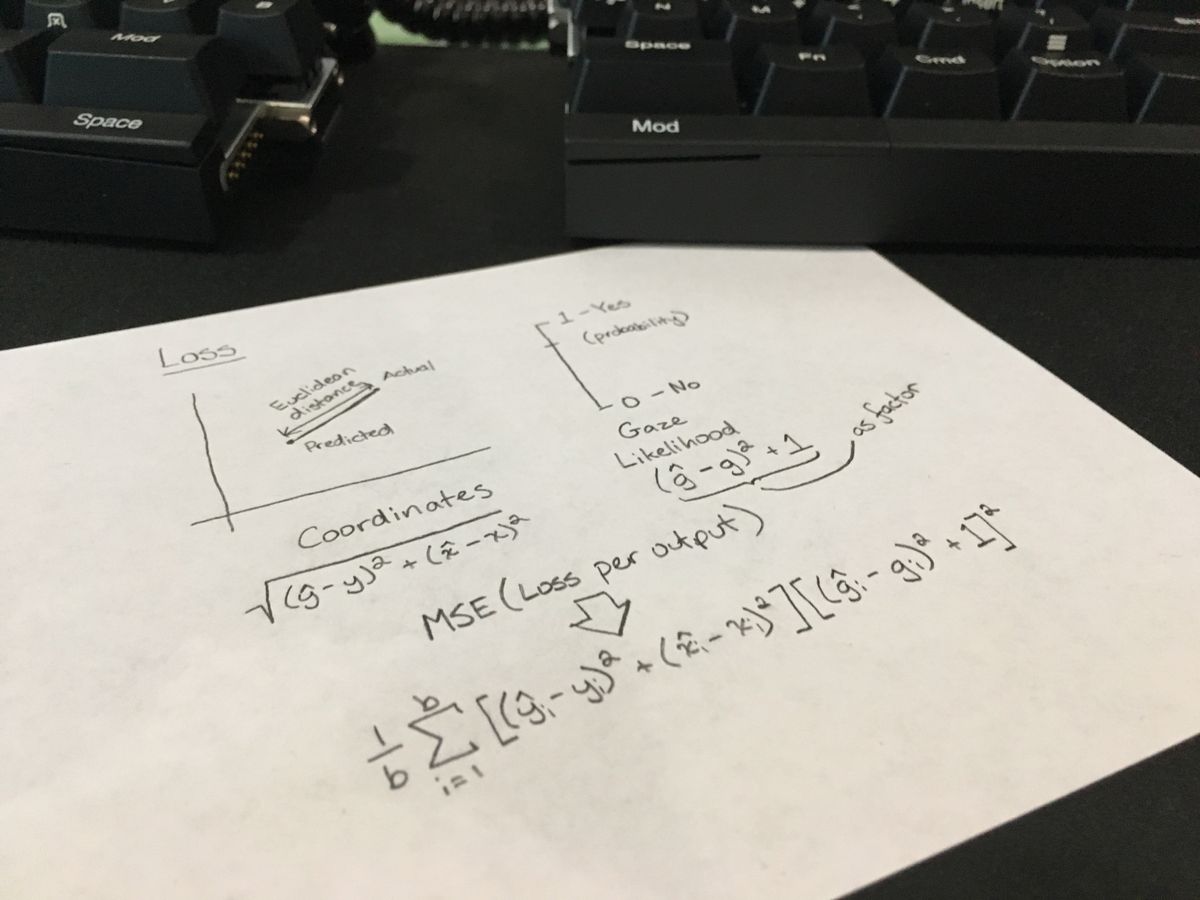
So, here's the problem. It's not terribly complicated to generate the probability as a value from 0 to 1. The more difficult piece is coming up with a single loss function that describes how "off" the prediction of the network really is. Prior to this point, I had been using the mean-squared error (MSE) of the distance between the predicted and actual points (a.k.a. Euclidean distance or Pythagorean theorem).

(Feel free to skip to the next section is math isn't your cup of tea; you won't miss much.)

Conceptually, the goal is to penalize that Euclidean distance by a factor that describes the difference in predicted versus actual probability that the coordinate is actually meaningful. If the network predicts that the coordinate matters but the truth is that one eye isn't visible, the loss should be described as the Euclidean distance times a factor larger than 1. The other requirement of this loss function is that the raw Euclidean distance should be returned if the probability output is perfectly correct. Putting these requisites together, a single equation can be determined by combining a probability delta between 1 and 2 (the factor) and the existing loss function. Here is one method of accomplishing this without the need of an absolute value operation.

\begin{aligned}
    \text{Loss} &= \text{MSE}(\text{Euclidean distance (D) and Gaze likelihood (G)})\\
    G &\in [0, 1]\; \text{(where 0 means one or more eyes are not visible)}\\\\
    G_{\text{Loss}} &= (\hat{G} - G)^2 + 1\; \text{(as multiplicative error factor)}\\
    D_{\text{Loss}} &= \sqrt{(\hat{y} - y)^2 + (\hat{x} - x)^2}\\
    \text{MSE} &= \frac{1}{b}\sum_{i=1}^b(\text{distance}^2)\\\\
    \text{Loss} &= \frac{1}{b}\sum_{i=1}^b\left[\left((\hat{{}_{i}G_L} - {}_{i}G_L)^2 + 1\right)\cdot\sqrt{(\hat{y_i} - y_i)^2 + (\hat{x_i} - x_i)^2}\right]^2\\
    &= \frac{1}{b}\sum_{i=1}^b\left((\hat{{}_{i}G_L} - {}_{i}G_L)^2 + 1\right)^2\cdot\left((\hat{y_i} - y_i)^2 + (\hat{x_i} - x_i)^2\right)
\end{aligned}

Additionally, here is the tensorflow implementation (which ironically looks a bit cleaner):

# (1/b) ∑^b_(i=1)([(^G-G)^2 + 1]^2 * [(^y - y)^2 + (^x - x)^2])
def loss_func(actual, pred):
    x_diff = tf.square(pred[:, 0] - actual[:, 0])
    y_diff = tf.square(pred[:, 1] - actual[:, 1])
    g_diff = tf.square(pred[:, 2] - actual[:, 2])

    return K.mean(tf.square(g_diff + 1) * (y_diff + x_diff))

Check Those Activation Functions

With the loss function in place, I was able to continue experimenting with simpler versions of proven image-based neural network designs like Inception and ResNet50. Unfortunately, for many iterations even before adding the third output, I could not get the loss to go below 28 but doggedly hovered around 28-33. Finally, when I began adding the third output, I realized that I had a sigmoid activation function for the (x, y) coordinate. For those not immediately familiar with this function, here is its graph:

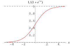
The problem is that it can never a value less than 0 or above 1! Feeling much humiliation after this silly mistake, I quickly adjusted the functions to use linear activation functions since the (x, y) coordinate is not technically limited to any particular range. (Although I could arbitrarily constrain it to the largest iOS device for this case since those are the only devices from GazeCapture, I have preferred to keep the neural network more general.)

Build, Measure, Learn

Throughout this process of output modification and loss adaption, I worked on various architectures. Although it is still too early to determine whether the discussed loss function will need tweaking, the current model training sessions have had measure of success though still limited. Many of the architecture iterations I was able to throw out quickly since the loss function was resulting in values in the trillions or quadrillions (even with the scale change of the new loss output which is much larger than 28-33).

With two GPUs (Nvidia 1080 Ti's) at my disposal in my custom build, I am currently running two slight variations of an architecture while measuring the results with TensorBoard as well as monitoring the output. I am still unsure about some of the results but am continuing to debug the extreme fluctuations that seem to occur in some of loss and val_loss outputs. Because many previous iterations have been upwards of 10^24 values, I am continuing with these models for a full 100 epoch cycle to see if they eventually converge.

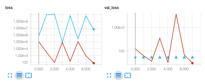
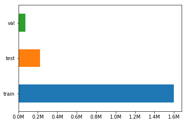
Although these results may not seem promising, several characteristics make v6 in particular (denoted by red) a bit more interesting. Per epoch, each model uses the entire available training set as well as the predetermined validation set established by the original GazeCapture researchers (where facial landmarks have been detected).

While the output of v6 seems to wildly vary per epoch, watching the results in person present a different story. The loss value steadily decreases perhaps 95% of the time and then spikes up by sometimes several orders of magnitude for remaining 5% of the time. The TensorBoard representation only captures the loss at the end of each epoch which only happens every ~1.5M rows (plus the validation set). The other consideration that must be made is that most of the activation functions need to use a linear activation function and do not therefore constrain the output of each neuron. I will just have to sit tight and wait to see how the model progresses especially considering the entire model right now is only 467KB.

# train.py (excerpt) - https://git.io/fxsO2

left_eye_input = Input(shape=(128,128,3))
right_eye_input = Input(shape=(128,128,3))
landmark_input = Input(shape=(68,3))

def eye_path(input_layer, prefix='na'):
    return pipe(
        input_layer,
        Conv2D(8, (3, 3), activation='relu', padding='same', name=(prefix + '_3x3conv1')),
        MaxPooling2D(pool_size=(3, 3), padding='same', name=(prefix + '_max1')),
        Conv2D(8, (3, 3), activation='relu', padding='same', name=(prefix + '_3x3conv2')),
        MaxPooling2D(pool_size=(3, 3), padding='same', name=(prefix + '_max2')),
        Conv2D(4, (2, 2), activation='relu', padding='same', name=(prefix + '_2x2conv1')),
        MaxPooling2D(pool_size=(2, 2), padding='same', name=(prefix + '_max3')),
        BatchNormalization(),
        Flatten(name=(prefix + '_flttn'))
    )


left_path = eye_path(left_eye_input, prefix='left')
right_path = eye_path(right_eye_input, prefix='right')

landmarks = pipe(
    landmark_input,
    Dense(16, activation='linear'),
    BatchNormalization(),
    Dense(8, activation='linear'),
    Flatten()
)

grouped = concatenate([left_path, right_path, landmarks])

coordinate = pipe(
    grouped,
    Dense(16, activation='linear'),
    Dense(8, activation='linear'),
    BatchNormalization(),
    Dense(2, activation='linear', name='coord_output')
)

gaze_likelihood = pipe(
    grouped,
    Dense(8, activation='relu'),
    BatchNormalization(),
    Dense(4, activation='relu'),
    Dense(1, activation='sigmoid', name='gaze_likelihood')
)
output = concatenate([coordinate, gaze_likelihood])

model = Model(inputs=[left_eye_input, right_eye_input, landmark_input],
              outputs=[output])

Thoughts or questions? Something not explained well? I am just starting into this deep learning world and would love to hear what you have to say.